How to build a profitable NQ strategy

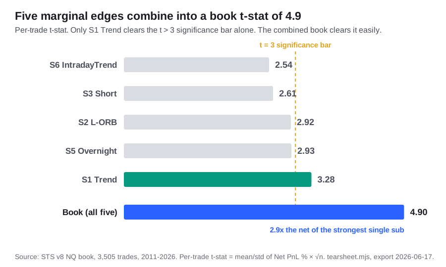
To build a profitable NQ strategy, stop hunting for one secret indicator and stack five honest edges instead: prove each edge is statistically real, stack edges that do not move together, size to survive a drawdown worse than any you have seen, prove it out of sample, and track it honestly. Those are the five steps, and we can show each one on a real 15-year book. Here is the number that carries the whole article: our five sub-strategies each have a per-trade t-stat between 2.54 and 3.28, and only one of them clears the usual t>3 significance bar alone. Combined, the book clears it at 4.9.

That gap, from a strongest single sub of 3.28 to a book of 4.9, is the entire point. You do not build a durable strategy by finding one perfect edge. You build it by stacking several honest, marginal edges that are nearly uncorrelated.

Whose trades are these

Six systematic NQ strategies, five active and one retired, share one single-position book. The window is June 2011 to June 2026. All numbers come from a TradingView List-of-Trades export dated 2026-06-17: 3,505 closed trades, $1,120,402 net on a fixed $100,000 basis, 45.5% win rate, profit factor 1.57. Sizing is 1 to 3 volatility-scaled mini contracts, commissions and slippage included, no compounding.

The style is momentum and trend-continuation: four intraday entries, one overnight, one short. Not mean reversion, not scalping. The five-step method transfers to any market. The exact numbers are this book's and are not universal constants.

The scorecard the rest of the article defends

Read the last two columns together. Four of five subs miss the t>3 bar on their own, and three of them (S3, S5, S6) have at least one 4-year era where profit factor dipped below 1.0. The book has neither problem. Its worst era still cleared 1.05, and its t-stat is 4.9.

Step 1: find a real edge, not a nice equity curve

A pretty backtest is easy to draw and easy to fool yourself with. The gate we use is stricter: a per-trade t-stat above 3, and a positive profit factor in every 4-year era, not just over the full run.

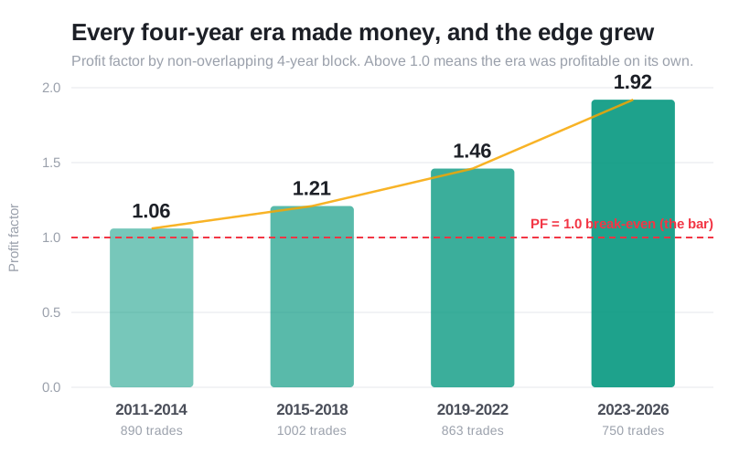
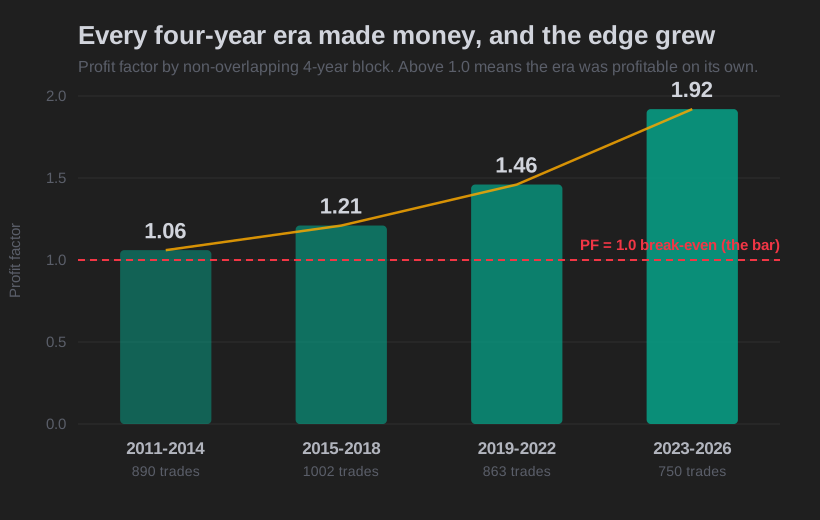
Profit factor is gross wins divided by gross losses. Our book clears both tests. Its per-trade t-stat is 4.9. Split the 15 years into rolling 4-year windows and every single era is profitable, from a low of about 1.05 up to 1.92. No era went underwater.

Now the honest part. Judged alone, only one of our five subs clears t>3: S1 Trend at 3.28. The other four land between 2.54 and 2.93. On their own, they are marginal edges, not slam dunks. We are not going to pretend otherwise, because the whole method depends on that being true.

Two honest caveats on that 4.9. First, it is an in-sample number, and these five subs were selected from a larger search (a sixth, S4, is already retired), so the raw t overstates the true edge once you account for the searching. Treat 4.9 as the optimistic end. Second, per-trade t treats all 3,505 trades as independent, but momentum trades cluster in the same sessions, so the effective sample is smaller than the raw count. The honest floor is the daily-return basis, which is less inflated by that clustering, and on it all five subs still clear 3.0 (they run 3.16 to 3.64).

Step 2: stack edges that do not move together

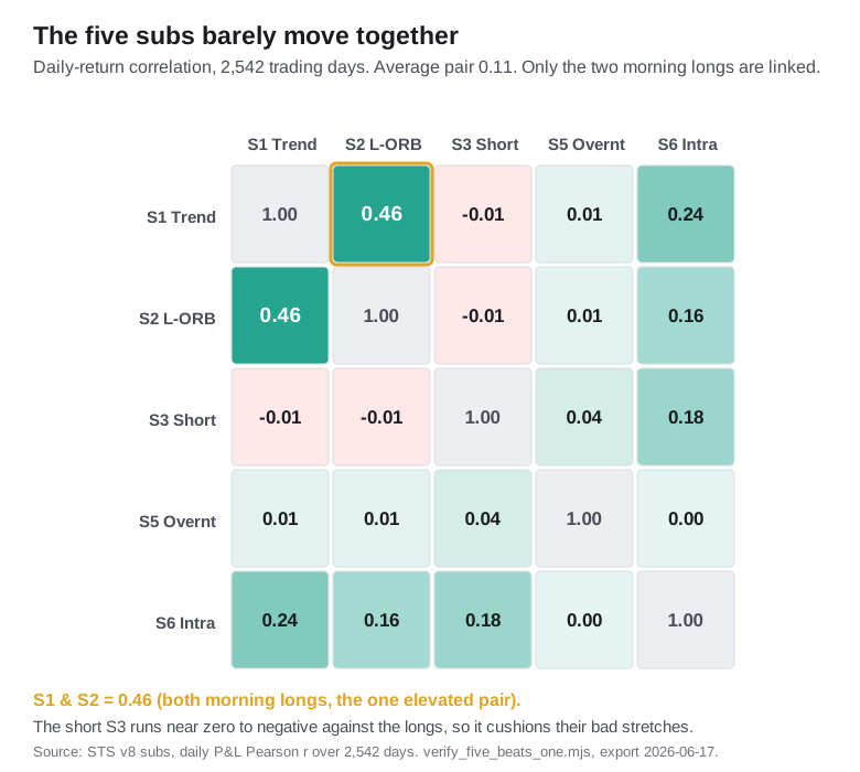
This is the step that turns five marginal subs into one strong book. Across 2,542 trading days, the average pairwise correlation between our subs is 0.11. That is close to independent.

The only elevated pair is S1 and S2, at 0.46, and that makes sense because both are morning longs. Everything else is low. The short, S3, runs near zero to slightly negative against the two morning longs: -0.01 against S1, -0.01 against S2. When the longs are having a rough stretch, the short is not automatically dragged down with them.

Near-independence is the main mechanism, helped by the larger combined sample. Correlations near 0.11 let five per-trade t-stats of 2.54 to 3.28 combine into a book t-stat of 4.9. It is the same reason a diversified fund beats a single stock: the edges are real, but their wobbles do not line up, so they partly cancel. The payoff is concrete. The book's net is 2.9 times the best single sub, and per dollar of max drawdown it returns about three times what the best single strategy does.

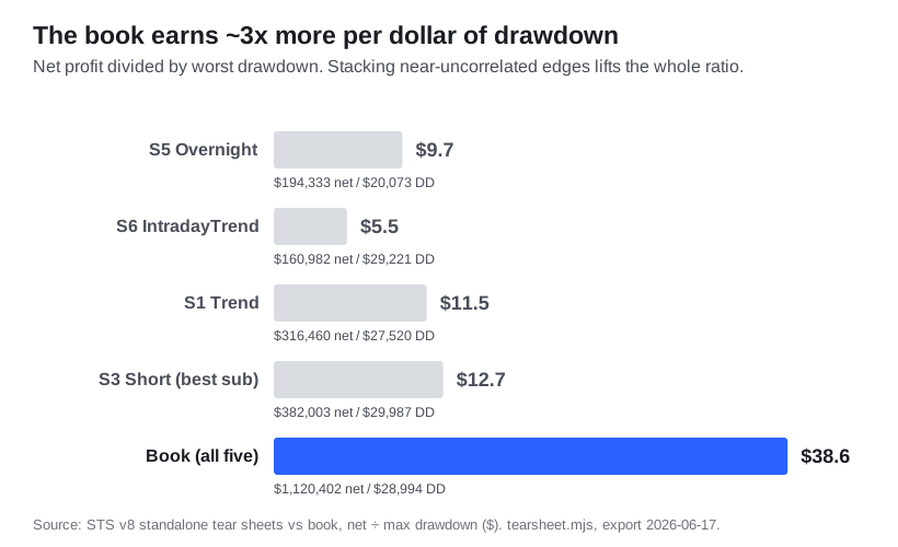
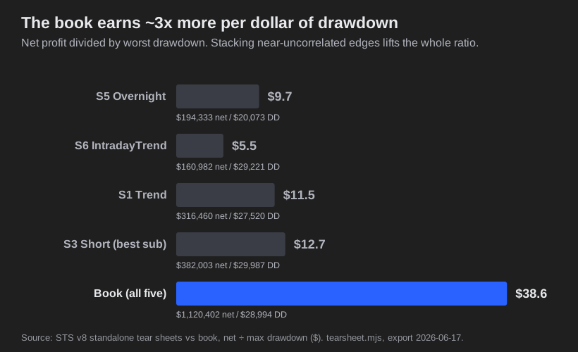
One caution on that best single sub. S3 Short earns its $12.7 return-per-drawdown on only 412 trades, the thinnest sample of the five, so its standalone ratio is the least certain of the group. The book's $38.6 does not lean on S3 alone, which is the point of stacking.

If any of these correlations spiked toward 1 in a crash, this step would fail. That is exactly what we watch for.

Step 3: size to survive variance, not to survive the backtest

Here is the trap. Our realized max drawdown is $28,994. That number is real, but it is also lucky. When we reshuffle the trade order 10,000 times, keeping each trade's actual profit and loss frozen, that $28,994 sits at about the 2nd percentile. Ninety-eight of a hundred reshuffles drew down more.

The median forward drawdown across those reshuffles is about $42,000. The 95th percentile is about $62,000. So the drawdown you should plan for is roughly 45% deeper than the one we actually lived through.

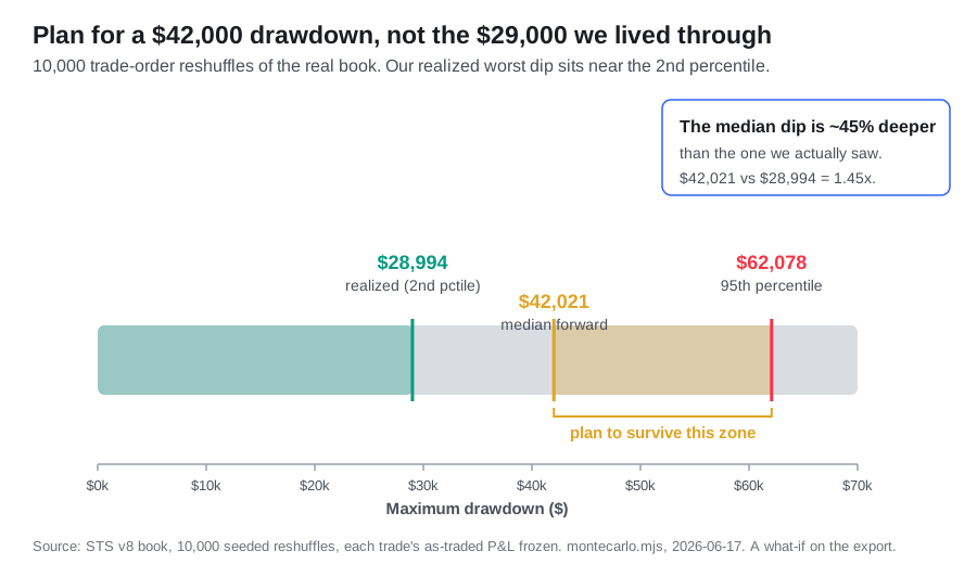
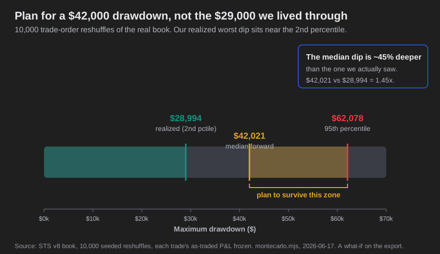
Size off the $42,000, not the $29,000. This has a hard practical edge. A $50,000 trailing-drawdown prop account cannot hold a book that can lose $42,000 or more and keep trading. That is the concrete reason we scale down to micro contracts: it keeps the worst plausible drawdown inside what an account can survive. The full case for planning around the deeper number is in expect worse drawdown than your backtest.

Step 4: prove it out of sample, do not tune it to the past

Overfitting is fitting a strategy so tightly to old data that it has nothing left for new data. Three checks keep us honest here; the full checklist is in is my backtest overfit.

First, per-era stability. The book's profit factor across rolling 4-year windows never drops below 1.0, and climbs from about 1.05 to 1.92. A curve-fit strategy usually has at least one era that falls apart. Ours does not, at the book level.

Second, recent out-of-sample. Every sub has been profitable since January 2026, with profit factors from 1.46 to 6.69. That is a small, recent sample, so we treat it as encouraging, not as proof.

Third, candor about the parts. Three subs (S3, S5, S6) each have a single 4-year era with a profit factor below 1.0, and four of five miss t>3 alone. We use round, natural parameters and we name the weak spots rather than hide them. If a sub with t>3 died out of sample, that would falsify this step.

Step 5: run it live and track it honestly

The track record is the product. So we publish the numbers that make us look worse, not just the ones that make us look good.

The clearest example is the drawdown gap from step 3. Our realized $28,994 is better than the $42,000 median we expect going forward. We publish that gap instead of quietly banking the lucky number. When the live sample grows, the honest test is whether the realized drawdown stays inside the Monte-Carlo band.

We also say plainly that four of five subs miss t>3 alone, and that some have a losing era. Most builders skip this step. An edge that passes steps 1 through 4 still has to survive the gap between backtest and live, and the only way to know is to run it and report what happens.

The build checklist you can paste into your notes

• Step 1: per-trade t-stat above 3 AND positive profit factor in every 4-year era. Not just a nice full-sample curve.
• Step 2: average pairwise correlation between your edges under about 0.3. If two edges move together, they count as roughly one.
• Step 3: size off your Monte-Carlo median drawdown, not your realized drawdown. Reshuffle trade order 10,000 times and read the median and 95th percentile.
• Step 4: out-of-sample positive, no sub-1.0 era at the book level, round parameters only.
• Step 5: publish realized-versus-expected, name the weak components, update on every contract roll.

To reproduce the per-sub gate on your own export, we ran one line per strategy:

node tearsheet.mjs <export.csv> "<name>"

That prints net, trades, profit factor, per-era PF, and the per-trade t-stat, which is everything you need for the step-1 and step-4 gates.

Methodology

• Instrument: NQ, the CME E-mini Nasdaq-100 futures, mini contract.
• Data and window: TradingView List-of-Trades export, 2011-06-24 to 2026-06-17, 15 years, 3,505 closed trades.
• Costs and sizing: commissions and slippage included in TradingView net PnL; 1 to 3 volatility-scaled contracts; fixed $100,000 basis; no compounding.
• t-stat basis: per-trade Net PnL percent, the stricter ruler. On a daily-return basis all five subs clear 3.0.
• Monte Carlo: 10,000 trade-order reshuffles with deterministic seeds, each trade's as-traded profit and loss frozen and re-ordered, never resized. We publish the historical point estimate as the headline and the reshuffle band only as a robustness check.
• What would falsify each step: step 1, a sub with t>3 that dies out of sample; step 2, correlations that spike toward 1 in a crash; step 3, a realized drawdown that already exceeds the reshuffle 95th percentile; step 4, an era profit factor that goes below 1.0 book-wide; step 5, a realized track that diverges from the backtest beyond the Monte-Carlo band.
• Independent re-derivation: every load-bearing number here was re-computed from the raw per-trade export by a second, from-scratch parser and calculation, and the leave-one-out drawdown attribution was re-run by two separate reconstructions. The book t-stat reproduced at 4.896, the drawdown at $28,994, and the drawdown-adder subs at S1 and S5.

One limit worth stating

The leave-one-out drawdown contributions here are offline approximations, built by subtracting each sub's standalone daily P&L from the book's daily P&L, not full in-engine 4-sub reruns. On this book, "every sub reduces the drawdown" is false: across three independent reconstructions of the stated method, dropping S1 or S5 lowers the book drawdown, which means those two subs are net drawdown-adders. The other three subs (S2, S3, S6) are the drawdown-reducers, S6 by the widest margin. The diversification lift on returns and on the t-stat is real and two-way verified. The claim that any single sub always shrinks the drawdown is not, so we do not make it. The Monte-Carlo band is also a what-if on the export, so it captures trade-ordering uncertainty only, not fill-model or slippage error, which means the real forward drawdown tail could run wider than the reshuffle band shows.

If you would rather run the finished book than build one, that is what we sell: see our five strategies and pricing. To go deeper on the individual steps, see our five NQ strategies explained for the diversification math, expect worse drawdown than your backtest for step 3, is my backtest overfit for step 4, and how to audit a trading track record for step 5.

What we test next

The step most builders skip is step 5, and it is the one we are still living through. An edge that passes steps 1 through 4 still has to survive live. The next thing we test is whether the realized forward drawdown stays inside the Monte-Carlo band as the live sample grows past the backtest.

Conflict disclosure: we trade this book live and we sell access to the signals. Judge the data accordingly.

CFTC Rule 4.41: Hypothetical or simulated performance results have certain limitations. Unlike an actual performance record, simulated results do not represent actual trading. Also, since the trades have not actually been executed, the results may have under- or over-compensated for the impact, if any, of certain market factors, such as lack of liquidity. Simulated trading programs in general are also subject to the fact that they are designed with the benefit of hindsight. No representation is being made that any account will or is likely to achieve profit or losses similar to those shown.

Past performance is not indicative of future results.